Using different MC packages for Bayesian sampling
refnx can work with a variety of MC packages for inference. This notebook will demonstrate the use of various packages:
An excellent reference to see how to use a wide range of packages for statistical inference is https://mattpitkin.github.io/samplers-demo/pages/samplers-samplers-everywhere.
import os
# Set these FIRST before any other imports
os.environ["JAX_ENABLE_X64"] = "1"

import warnings
from importlib import resources
import numpy as np
import matplotlib.pyplot as plt
import scipy
import multiprocessing as mp

from jax import config
config.update("jax_enable_x64", True)
warnings.filterwarnings("ignore", message="Numba will use object mode", category=UserWarning)


import refnx
from refnx.dataset import ReflectDataset, Data1D
from refnx.analysis import (
    Transform,
    CurveFitter,
    Objective,
    Model,
    Parameter,
    pymc_model,
    process_chain,
)
from refnx.reflect import SLD, Slab, ReflectModel

import pymc as pm
import dynesty
import arviz as az
It’s important to note down the versions of the software that you’re using, in order for the analysis to be reproducible.
print(
    f"refnx: {refnx.version.version}\n"
    f"scipy: {scipy.version.version}\n"
    f"numpy: {np.version.version}"
)
refnx: 0.1.66.dev0+git20260720.f8a4254
scipy: 1.18.0
numpy: 2.4.6
The dataset we’re going to use as an example is distributed with every install. The following cell determines its location.
pth = resources.files(refnx.analysis)
DATASET_NAME = "c_PLP0011859_q.txt"
file_path = pth / f"tests/{DATASET_NAME}"

data = ReflectDataset(file_path)
The Structure
si = SLD(2.07, name="Si")
sio2 = SLD(3.47, name="SiO2")
film = SLD(2.0, name="film")
d2o = SLD(6.36, name="d2o")
# first number is thickness, second number is roughness
# a native oxide layer
sio2_layer = sio2(30, 3)

# the film of interest
film_layer = film(250, 3)

# layer for the solvent
d2o_layer = d2o(0, 3)
sio2_layer.thick.setp(bounds=(15, 50), vary=True)
sio2_layer.rough.setp(bounds=(1, 15), vary=True)

film_layer.thick.setp(bounds=(200, 300), vary=True)
film_layer.sld.real.setp(bounds=(0.1, 3), vary=True)
film_layer.rough.setp(bounds=(1, 15), vary=True)

d2o_layer.rough.setp(vary=True, bounds=(1, 15))
structure = si | sio2_layer | film_layer | d2o_layer
print(sio2_layer.parameters)
________________________________________________________________________________
Parameters:     'SiO2'
<Parameter:'SiO2 - thick' , value=30          , bounds=[15.0, 50.0]>
________________________________________________________________________________
Parameters:     'SiO2'
<Parameter: 'SiO2 - sld'  , value=3.47  (fixed) , bounds=[-inf, inf]>
<Parameter: 'SiO2 - isld' , value=0  (fixed) , bounds=[-inf, inf]>
<Parameter:'SiO2 - rough' , value=3          , bounds=[1.0, 15.0]>
<Parameter:'SiO2 - volfrac solvent', value=0  (fixed) , bounds=[0.0, 1.0]>
ReflectModel, Objective, Curvefitter
model = ReflectModel(structure, bkg=3e-6, dq=5.0)
model.scale.setp(bounds=(0.6, 1.2), vary=True)
model.bkg.setp(bounds=(1e-9, 9e-6), vary=True)
objective = Objective(model, data, transform=Transform("logY"))
fitter = CurveFitter(objective)
fitter.fit("differential_evolution", target="nlpost");
-564.1887453974779: : 51it [00:02, 19.06it/s]
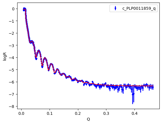
objective.plot()
plt.legend()
plt.xlabel("Q")
plt.ylabel("logR")
plt.legend();
emcee
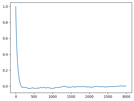
Now lets do a MCMC sampling of the curvefitting system. First we do sampling to burn-in the system. We’ll also checkout the autocorrelation time of the system. We’ll then discard the burn-in samples because the initial chain might not be representative of an equilibrated system (i.e. distributed around the mean with the correct covariance).
fitter.sample(3000, pool=-1);
100%|████████████████████████████████████████████████████████████████████████████████████████████████████████████████████████████████████████████████████████| 3000/3000 [02:11<00:00, 22.83it/s]
plt.plot(fitter.acf()[:, 4])
fitter.reset()
We then follow up with a production run, only saving 1 in 200 samples. This is to remove autocorrelation. We save 15 steps, giving a total of 15 * 200 samples (200 walkers is the default).
res = fitter.sample(15, nthin=200, pool=-1)
100%|████████████████████████████████████████████████████████████████████████████████████████████████████████████████████████████████████████████████████████| 3000/3000 [02:12<00:00, 22.61it/s]
This seems to be an effective sampling rate of ~15 * 200 / 132 = 23 samples/sec
In the final output of the sampling each varying parameter is given a set of statistics. Parameter.value is the median of the chain samples. Parameter.stderr is half the [15, 85] percentile, representing a standard deviation.
print(objective)
________________________________________________________________________________
Objective - 5224508656
Dataset = c_PLP0011859_q
datapoints = 408
chi2 = 919.5927464121912
Weighted = True
Transform = Transform('logY')
________________________________________________________________________________
Parameters:       ''
________________________________________________________________________________
Parameters: 'instrument parameters'
<Parameter:    'scale'    , value=0.87943 +/- 0.00304, bounds=[0.6, 1.2]>
<Parameter:     'bkg'     , value=4.59101e-07 +/- 2.24e-08, bounds=[1e-09, 9e-06]>
<Parameter:'dq - resolution', value=5  (fixed) , bounds=[-inf, inf]>
<Parameter:  'q_offset'   , value=0  (fixed) , bounds=[-inf, inf]>
________________________________________________________________________________
Parameters: 'Structure - '
________________________________________________________________________________
Parameters:      'Si'
<Parameter: 'Si - thick'  , value=0  (fixed) , bounds=[-inf, inf]>
________________________________________________________________________________
Parameters:      'Si'
<Parameter:  'Si - sld'   , value=2.07  (fixed) , bounds=[-inf, inf]>
<Parameter:  'Si - isld'  , value=0  (fixed) , bounds=[-inf, inf]>
<Parameter: 'Si - rough'  , value=0  (fixed) , bounds=[-inf, inf]>
<Parameter:'Si - volfrac solvent', value=0  (fixed) , bounds=[0.0, 1.0]>
________________________________________________________________________________
Parameters:     'SiO2'
<Parameter:'SiO2 - thick' , value=38.6306 +/- 0.374, bounds=[15.0, 50.0]>
________________________________________________________________________________
Parameters:     'SiO2'
<Parameter: 'SiO2 - sld'  , value=3.47  (fixed) , bounds=[-inf, inf]>
<Parameter: 'SiO2 - isld' , value=0  (fixed) , bounds=[-inf, inf]>
<Parameter:'SiO2 - rough' , value=5.83214 +/- 0.301, bounds=[1.0, 15.0]>
<Parameter:'SiO2 - volfrac solvent', value=0  (fixed) , bounds=[0.0, 1.0]>
________________________________________________________________________________
Parameters:     'film'
<Parameter:'film - thick' , value=259.04 +/- 0.251, bounds=[200.0, 300.0]>
________________________________________________________________________________
Parameters:     'film'
<Parameter: 'film - sld'  , value=2.40186 +/- 0.0125, bounds=[0.1, 3.0]>
<Parameter: 'film - isld' , value=0  (fixed) , bounds=[-inf, inf]>
<Parameter:'film - rough' , value=8.8294 +/- 0.36 , bounds=[1.0, 15.0]>
<Parameter:'film - volfrac solvent', value=0  (fixed) , bounds=[0.0, 1.0]>
________________________________________________________________________________
Parameters:      'd2o'
<Parameter: 'd2o - thick' , value=0  (fixed) , bounds=[-inf, inf]>
________________________________________________________________________________
Parameters:      'd2o'
<Parameter:  'd2o - sld'  , value=6.36  (fixed) , bounds=[-inf, inf]>
<Parameter: 'd2o - isld'  , value=0  (fixed) , bounds=[-inf, inf]>
<Parameter: 'd2o - rough' , value=3.78935 +/- 0.111, bounds=[1.0, 15.0]>
<Parameter:'d2o - volfrac solvent', value=0  (fixed) , bounds=[0.0, 1.0]>
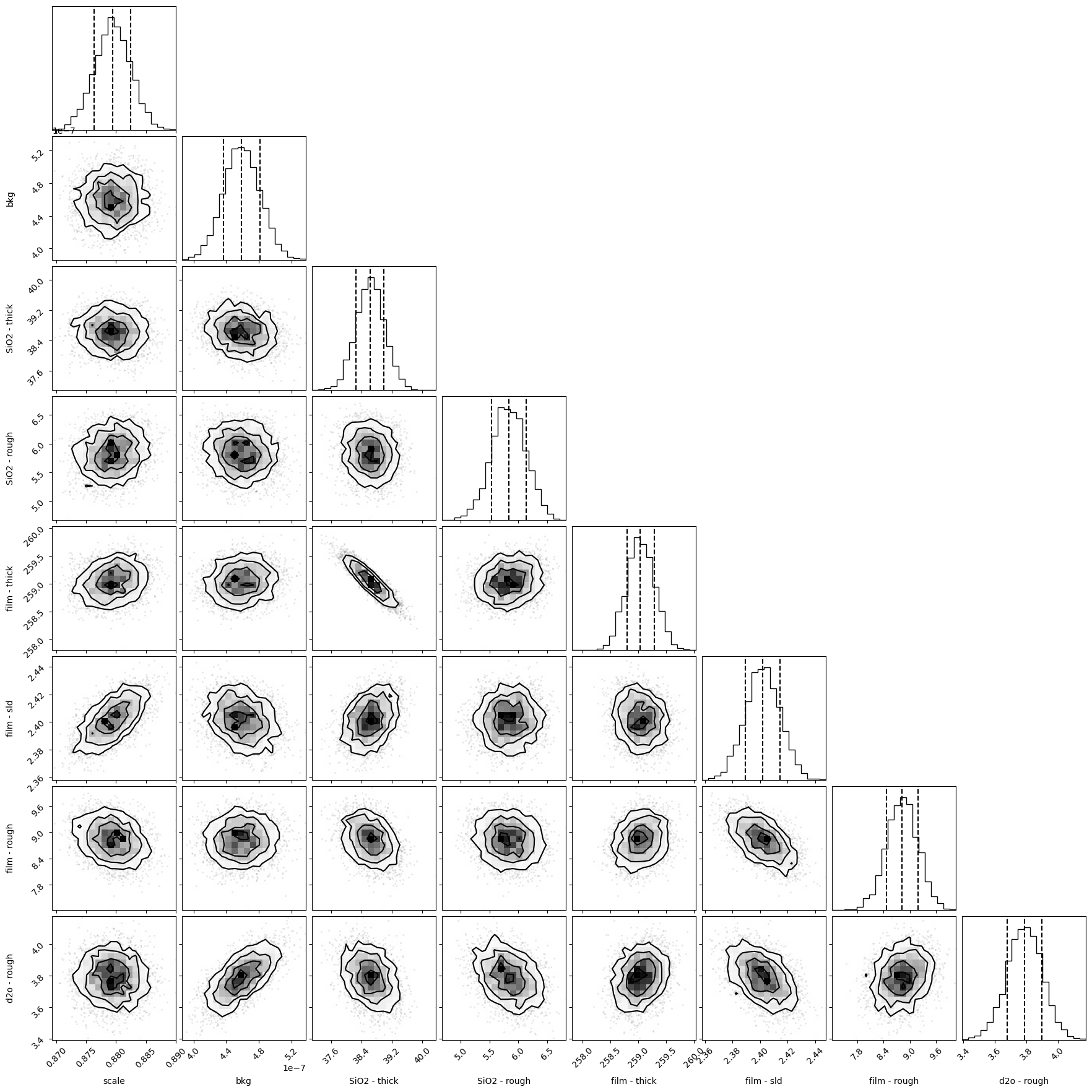
A corner plot shows the covariance between parameters. You need to install the matplotlib and corner packages to create these graphs.
objective.corner();
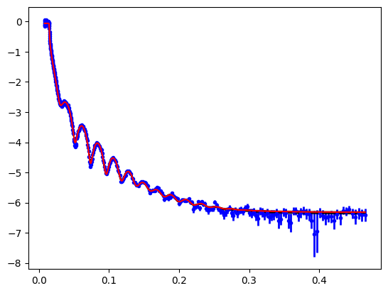
Once we’ve done the sampling we can look at the variation in the model at describing the data. In this example there isn’t much spread.
objective.plot(samples=300);
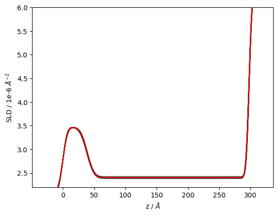
In a similar manner we can look at the spread in SLD profiles consistent with the data.
structure.plot(samples=300)
plt.ylim(2.2, 6);
Sampling with pymc
pymc is also an excellent Bayesian package. refnx has some features built in to work with pymc models. You’ll need to install pymc, pytensor, and arviz to run this section.
from refnx.reflect.extra import to_pymc_model
import pymc as pm
import arviz as az
refnx can now use the NUTS sampler, which is high performance.
_model = to_pymc_model(objective)
with _model:
    idata = pm.sample(mp_ctx=mp.get_context("forkserver"))
Initializing NUTS using jitter+adapt_diag...
Multiprocess sampling (4 chains in 4 jobs)
NUTS: [p0, p1, p2, p3, p4, p5, p6, p7]
/Users/andrew/.conda/envs/dev3/lib/python3.14/site-packages/pytensor/link/numba/dispatch/basic.py:234: UserWarning: Numba will use object mode to run _LogLikeValueGradOp's perform method. Set `pytensor.config.compiler_verbose = True` to see more details.
  warnings.warn(
/Users/andrew/.conda/envs/dev3/lib/python3.14/site-packages/pytensor/link/numba/dispatch/basic.py:234: UserWarning: Numba will use object mode to run _LogLikeValueGradOp's perform method. Set `pytensor.config.compiler_verbose = True` to see more details.
  warnings.warn(
/Users/andrew/.conda/envs/dev3/lib/python3.14/site-packages/pytensor/link/numba/dispatch/basic.py:234: UserWarning: Numba will use object mode to run _LogLikeValueGradOp's perform method. Set `pytensor.config.compiler_verbose = True` to see more details.
  warnings.warn(
/Users/andrew/.conda/envs/dev3/lib/python3.14/site-packages/pytensor/link/numba/dispatch/basic.py:234: UserWarning: Numba will use object mode to run _LogLikeValueGradOp's perform method. Set `pytensor.config.compiler_verbose = True` to see more details.
  warnings.warn(
Sampling 4 chains for 1_000 tune and 1_000 draw iterations (4_000 + 4_000 draws total) took 141 seconds.
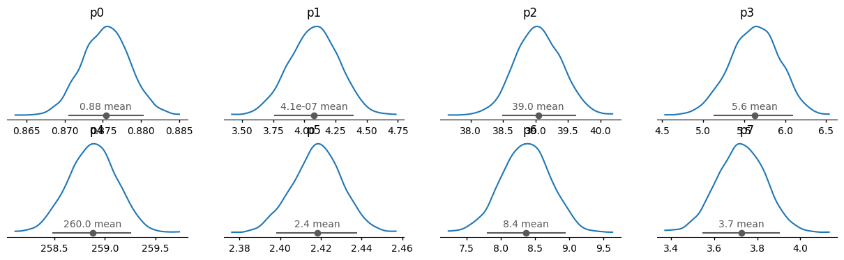
az.plot_dist(idata);
az.plot_autocorr(idata, max_lag=1000);
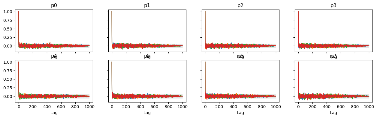
The autocorrelation time is 0, so we have a total of 4000 independent samples (1000 on each of the 4 chains). The time taken on my machine was ~146 sec, which includes tuning time. This is an effective sampling rate of 27 samples/sec.
Note how all the parameters are labelled p0, p1, ..., pn. Each of those parameters correspond to a Parameter in Objective.varying_parameters(). Let’s do some processing to update the objective with the sampling results.
# bring the pymc traces back into the Objective.
npars = len(objective.varying_parameters())
total_chain = [idata.posterior[f'p{i}'].to_numpy() for i in range(npars)]
tc = np.r_[total_chain]
process_chain(objective, np.swapaxes(tc, 0, 2));
print(objective)
________________________________________________________________________________
Objective - 5224508656
Dataset = c_PLP0011859_q
datapoints = 408
chi2 = 940.1710447120929
Weighted = True
Transform = Transform('logY')
________________________________________________________________________________
Parameters:       ''
________________________________________________________________________________
Parameters: 'instrument parameters'
<Parameter:    'scale'    , value=0.875423 +/- 0.00305, bounds=[0.6, 1.2]>
<Parameter:     'bkg'     , value=4.08174e-07 +/- 2e-08, bounds=[1e-09, 9e-06]>
<Parameter:'dq - resolution', value=5  (fixed) , bounds=[-inf, inf]>
<Parameter:  'q_offset'   , value=0  (fixed) , bounds=[-inf, inf]>
________________________________________________________________________________
Parameters: 'Structure - '
________________________________________________________________________________
Parameters:      'Si'
<Parameter: 'Si - thick'  , value=0  (fixed) , bounds=[-inf, inf]>
________________________________________________________________________________
Parameters:      'Si'
<Parameter:  'Si - sld'   , value=2.07  (fixed) , bounds=[-inf, inf]>
<Parameter:  'Si - isld'  , value=0  (fixed) , bounds=[-inf, inf]>
<Parameter: 'Si - rough'  , value=0  (fixed) , bounds=[-inf, inf]>
<Parameter:'Si - volfrac solvent', value=0  (fixed) , bounds=[0.0, 1.0]>
________________________________________________________________________________
Parameters:     'SiO2'
<Parameter:'SiO2 - thick' , value=39.0362 +/- 0.354, bounds=[15.0, 50.0]>
________________________________________________________________________________
Parameters:     'SiO2'
<Parameter: 'SiO2 - sld'  , value=3.47  (fixed) , bounds=[-inf, inf]>
<Parameter: 'SiO2 - isld' , value=0  (fixed) , bounds=[-inf, inf]>
<Parameter:'SiO2 - rough' , value=5.6366 +/- 0.303, bounds=[1.0, 15.0]>
<Parameter:'SiO2 - volfrac solvent', value=0  (fixed) , bounds=[0.0, 1.0]>
________________________________________________________________________________
Parameters:     'film'
<Parameter:'film - thick' , value=258.88 +/- 0.241, bounds=[200.0, 300.0]>
________________________________________________________________________________
Parameters:     'film'
<Parameter: 'film - sld'  , value=2.41852 +/- 0.0121, bounds=[0.1, 3.0]>
<Parameter: 'film - isld' , value=0  (fixed) , bounds=[-inf, inf]>
<Parameter:'film - rough' , value=8.3713 +/- 0.356, bounds=[1.0, 15.0]>
<Parameter:'film - volfrac solvent', value=0  (fixed) , bounds=[0.0, 1.0]>
________________________________________________________________________________
Parameters:      'd2o'
<Parameter: 'd2o - thick' , value=0  (fixed) , bounds=[-inf, inf]>
________________________________________________________________________________
Parameters:      'd2o'
<Parameter:  'd2o - sld'  , value=6.36  (fixed) , bounds=[-inf, inf]>
<Parameter: 'd2o - isld'  , value=0  (fixed) , bounds=[-inf, inf]>
<Parameter: 'd2o - rough' , value=3.72596 +/- 0.112, bounds=[1.0, 15.0]>
<Parameter:'d2o - volfrac solvent', value=0  (fixed) , bounds=[0.0, 1.0]>
The parameter values from pymc and emcee are effectively the same.
Sampling with dynesty
import dynesty
You can find out how to estimate posteriors with dynesty using this page, https://dynesty.readthedocs.io/en/stable/dynamic.html. It’s best to use the dynamic nested sampler, then you need to reweight the samples with the weights. Dynesty provides a utility function for that. You can also use dynesty to perform model comparison by looking at the evidence term.
nested_sampler = dynesty.DynamicNestedSampler(
    objective.logl, objective.prior_transform, ndim=len(objective.varying_parameters())
)
nested_sampler.run_nested()
# process the samples
chain = nested_sampler.results.samples_equal()

# another way of processing the samples (reweighting is needed)
logZdynesty = nested_sampler.results.logz[-1]  # value of logZ
weights = np.exp(nested_sampler.results.logwt - logZdynesty)
chain = dynesty.utils.resample_equal(nested_sampler.results.samples, weights)

print(chain.shape)
26892it [00:59, 449.86it/s, batch: 5 | bound: 13 | nc: 1 | ncall: 117209 | eff(%): 22.837 | loglstar: 563.323 < 570.721 < 569.050 | logz: 536.576 +/- 0.190 | stop: 0.878]
(26892, 8)
The size of the chain resulting from the samples_equal method is not equal to the number of effective samples. One can estimate the effective number of posterior samples resulting from a run using the following:
def ess(weights):
    """
    Estimate the effective sample size from the weights.

    Args:
        weights (array_like): an array of weights values for each nested sample

    Returns:
        int: the effective sample size
    """

    N = len(weights)
    w = weights / weights.sum()
    ess = N / (1.0 + ((N * w - 1) ** 2).sum() / N)

    return int(ess)


print("effective number of samples: ", ess(np.exp(weights)))
effective number of samples: 26891
The effective sampling rate for dynesty seems to be ~26048/61 ~ 427 samples/sec.
Let’s process the chain to put the statistics into the objective. Here we’ll use the process_chain utility function that’s designed for use with emcee chains. This function assumes that the chain has shape (nsteps, nwalkers, nvars). The chain from dynesty has shape (nsamples, nvars), so we can fake the dynesty chain into looking like an emcee chain by putting an extra axis in.
process_chain(objective, chain[:, None, :]);
print(objective)
________________________________________________________________________________
Objective - 5224508656
Dataset = c_PLP0011859_q
datapoints = 408
chi2 = 919.5914183460201
Weighted = True
Transform = Transform('logY')
________________________________________________________________________________
Parameters:       ''
________________________________________________________________________________
Parameters: 'instrument parameters'
<Parameter:    'scale'    , value=0.879414 +/- 0.00305, bounds=[0.6, 1.2]>
<Parameter:     'bkg'     , value=4.59504e-07 +/- 2.28e-08, bounds=[1e-09, 9e-06]>
<Parameter:'dq - resolution', value=5  (fixed) , bounds=[-inf, inf]>
<Parameter:  'q_offset'   , value=0  (fixed) , bounds=[-inf, inf]>
________________________________________________________________________________
Parameters: 'Structure - '
________________________________________________________________________________
Parameters:      'Si'
<Parameter: 'Si - thick'  , value=0  (fixed) , bounds=[-inf, inf]>
________________________________________________________________________________
Parameters:      'Si'
<Parameter:  'Si - sld'   , value=2.07  (fixed) , bounds=[-inf, inf]>
<Parameter:  'Si - isld'  , value=0  (fixed) , bounds=[-inf, inf]>
<Parameter: 'Si - rough'  , value=0  (fixed) , bounds=[-inf, inf]>
<Parameter:'Si - volfrac solvent', value=0  (fixed) , bounds=[0.0, 1.0]>
________________________________________________________________________________
Parameters:     'SiO2'
<Parameter:'SiO2 - thick' , value=38.6345 +/- 0.369, bounds=[15.0, 50.0]>
________________________________________________________________________________
Parameters:     'SiO2'
<Parameter: 'SiO2 - sld'  , value=3.47  (fixed) , bounds=[-inf, inf]>
<Parameter: 'SiO2 - isld' , value=0  (fixed) , bounds=[-inf, inf]>
<Parameter:'SiO2 - rough' , value=5.83151  +/- 0.3 , bounds=[1.0, 15.0]>
<Parameter:'SiO2 - volfrac solvent', value=0  (fixed) , bounds=[0.0, 1.0]>
________________________________________________________________________________
Parameters:     'film'
<Parameter:'film - thick' , value=259.043 +/- 0.245, bounds=[200.0, 300.0]>
________________________________________________________________________________
Parameters:     'film'
<Parameter: 'film - sld'  , value=2.40197 +/- 0.0128, bounds=[0.1, 3.0]>
<Parameter: 'film - isld' , value=0  (fixed) , bounds=[-inf, inf]>
<Parameter:'film - rough' , value=8.8279 +/- 0.354, bounds=[1.0, 15.0]>
<Parameter:'film - volfrac solvent', value=0  (fixed) , bounds=[0.0, 1.0]>
________________________________________________________________________________
Parameters:      'd2o'
<Parameter: 'd2o - thick' , value=0  (fixed) , bounds=[-inf, inf]>
________________________________________________________________________________
Parameters:      'd2o'
<Parameter:  'd2o - sld'  , value=6.36  (fixed) , bounds=[-inf, inf]>
<Parameter: 'd2o - isld'  , value=0  (fixed) , bounds=[-inf, inf]>
<Parameter: 'd2o - rough' , value=3.78874 +/- 0.116, bounds=[1.0, 15.0]>
<Parameter:'d2o - volfrac solvent', value=0  (fixed) , bounds=[0.0, 1.0]>
Conclusions
Hopefully you’ve found it useful to see how the three sampling packages can be used to obtain posterior distributions for the parameter set. All have high performance.